


Ulysses HISCALE Data Analysis Handbook
Appendix 10. Effect of Backscattered Electrons on the Geometric Factors of the LEMS30 Telescope (Hong MS Thesis)

where ΔA'ij is the effective area of ΔAi (see Figure A10-7) looking into the solid angle of ΔΩij. ΔΩij is the solid angle of the jth escaped electron trajectory; n is the total number of finite areas ΔAi, and npas is the total number of escaped trajectories for ΔAi (see Section A10-6 for detailed derivations). To calculate the Ωij one can trace an electron starting from the open aperture with a particular energy and see if it can reach the area ΔAi of the detector. We also can do it time-reversed, starting at the center of ΔAi and trace its trajectory to see if it escapes the open aperture. In this project we use the second procedure. Since we would compare the results of the effect of backscattering electrons on geometric factors of LEMS 30 to Buckley's non-scattering results, it is important to use his model of calculation. The procedure is outlined as follows:
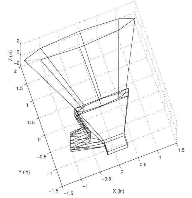
1) The telescope has a complex geometric shape. In order to determine the fate of a particle's trajectory (check if the particle should continue its trajectory) we need a simulation of the geometry of the telescope. Buckley modeled the whole LEMS 30 subsystem with plane polygons (see Figures A10-4 - A10-5). A complete listing of the coordinates of each vertex and coefficients of each plane can be found in Section A9.5.
Figure A10-4 View angle θ=0°, Φ=90°
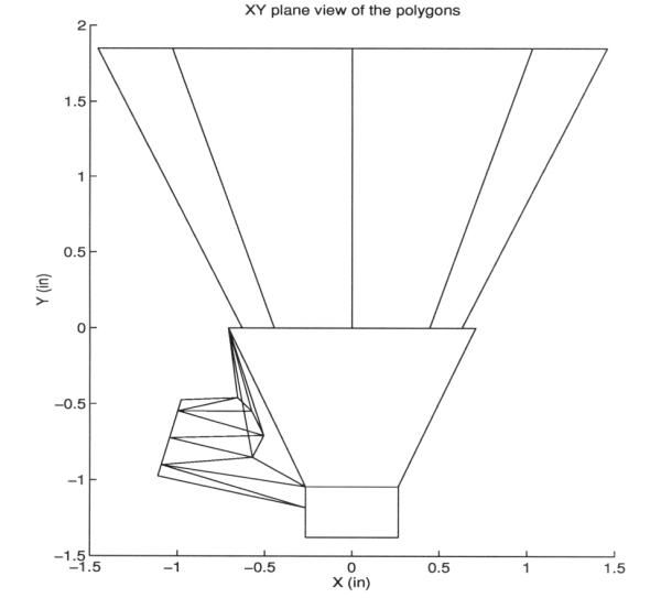
Figure A10-5 View angle θ=-20°, Φ=80°
2) The approximation of the magnetic field generated by the magnets is also needed. Buckley adapted Shodhan's model (Shodhan, S., Masters Thesis, Univ. of Kansas, 1988) to do the calculation for the LEMS 30 telescope.
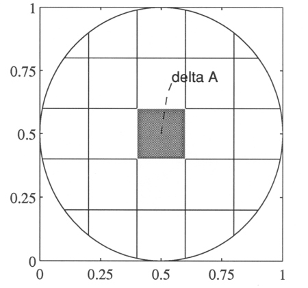
3) Divide the detector sensor into 21 small areas of ΔAi (see Figure A10-6). Choose a ΔAi. (For the coordinates of the center and area of each ΔAi see section 9.6.)
Figure A10-6 The detector is divided into 21 small ΔAi.
4) Start from the center of the small area ΔAi, choose initial θ0 and Φ0 with a particular energy for a small time interval (Δtj). During the time interval the particle moves from (xj, yj, zj) to (xj+1, yj+1, zj+1) under the influence of the magnetic field.
5) Determine whether the line segment formed by (xj, yj, zj) and (xj+1, yj+1, zj+1) has an intersection with any plane of the polygons of 1.
- If there is no intersection then calculate the trajectory of the electron for the time interval (Δtj+1); repeat step 5.
- If there is an intersection between the line segment
and a polygon then check to determine if the polygon is
the open aperture polygon.
- If it is open aperture, then terminate the trajectory because the electron escapes the open aperture.
- If it is not, then determine if the trajectory
has any earlier impact with the telescope.
- If there is no earlier impact, use a particular backscattering model (see Section A10.2) to reschedule the trajectory after the impact.
- If there was an earlier impact, then terminate the trajectory and the electron fails to be detected.
6) Repeat step 4 with change of Δθ and ΔΦ until it exhausts all possible combinations of θ and Φ.
7) Pick another ΔAi and repeat step 4. Notice that because of the symmetry of the detector we only need to pick ΔAi in a half of the detector. The results of the other half should be the same (see Figure A10-7).
Figure A10-7 The number of escapes at each ΔAi for energy of 50 keV (Radzimski's η is used).
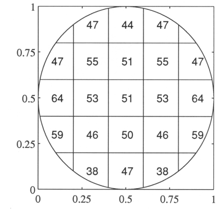
Figure A10-7 shows the number of escapes for energy of 50 keV for the electrons starting from the center of each ΔAi when Radzimski's backscattering coefficients are used. The results include elastic specular single backscattering electrons. More results can be found in Section A10.9 for both Radzimski's and Neubert's η and other energies.
8) One can use the results for the particular energy of the electrons to calculate the geometric factor by using the following formula:
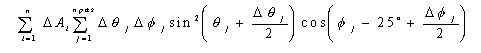
where n is total number of ΔAi's on the detector, ΔAi is the area of the i-th element on the detector, Δθj is the interval at which the polar angle is chosen to scan through the whole solid angles, θj and Φj are the polar and azimuthal angles at which the j-th electron starts from the center of the area which escapes the open aperture, and npas is the number of trajectories which reach the open aperture. The 25º that appears in the argument of cosine is needed because the detector B surface tilts in this coordinate system. See Section A10.6 for more details.
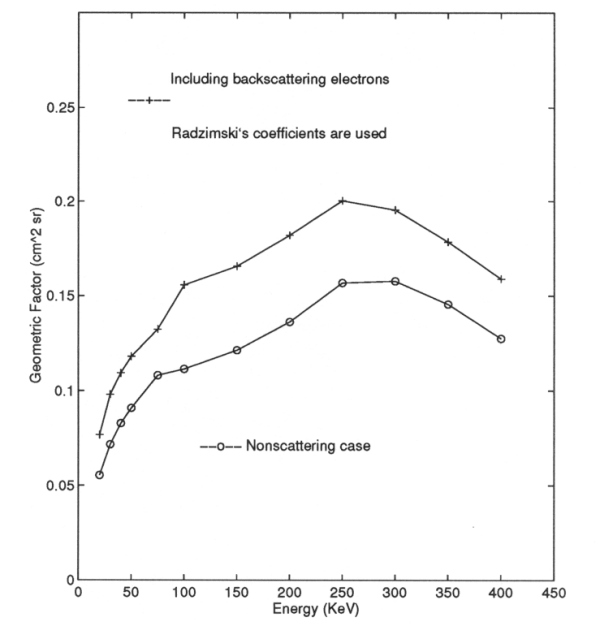
One can repeat all the above procedures to obtain the geometric factors for different energies. Shown in Figure A10-8 are the geometric factors vs. energies for including elastic specular single backscattering when Radsimski's η is used.
For details of the programming and codes see Section A10.8 and Section A10.11.
Figure A10-8 The geometric factor including specular backscattering; Radzimski's η is used.
Next: A10.4 Chapter 4 - Results and Discussion
Return to the Table of Contents for Hong's MS Thesis
Return to HISCALE List of Appendices
Return to Ulysses HISCALE Data Analysis Handbook Table of Contents
Updated 8/8/19, Cameron Crane
QUICK FACTS
Mission End Date: June 30, 2009
Destination: The inner heliosphere of the sun away from the ecliptic plane
Orbit: Elliptical orbit transversing the polar regions of the sun outside of the ecliptic plane