Current Location: NASA Science Support >> HISCALE Data Analysis Handbook >> Appendix 6

ULYSSES

Ulysses HISCALE Data Analysis Handbook

 

Appendix 6. Quality Controlled Averaging

 

The following appendix lists a memo to the HISCALE Investigation Team from Tom Armstrong and Dennis Haggerty about the HISCALE averages corrected for noise.

 

1.) The Problem

 

It has been obvious from the beginning of HISCALE data production that the HISCALE rates are on frequent occasions corrupted by false values that we presume are introduced between the accumulation of the count rates aboard Ulysses by the HISCALE instrument and the Experiment Data Records (EDR) generated by the JPL project data records system. Examples of the problems can be seen as "spikes" in the hourly averaged and spin averaged rates displayed in the plots that follow. The severity of the problem is variable. It is most noticeable in channels that have low intrinsic rates. It also appears to be episodic in time--that is, there are long periods where nearly all channels look fine and then multiple channels will be corrupted during the same limited time period. The nature of the data suggests that the noise introduces spurious high values of accumulated counts. In fact, close examination of representative cases shows a pattern of repeated (duplicate, two or three times) spuriously high values. The prevalence of noise in our count rates renders all "features" in daily averages, for example, suspect. In fact, for the low count rate channels, most of the daily averages computed up to this time are not trustworthy.

 

2.) Rationale in the Formulation of a Solution

 

Our goal is to produce trustworthy time averages--not to "correct" the data. That is, we shall regard it as sufficient to introduce a step which evaluates the numbers to be averaged and eliminates those which are suspect (not attempting to "correct" them) while retaining all of the naturally (correct) variation including trends which inevitably occur during the period being averaged. After considering and rejecting maximum rate checking and running filters based on trends, we have selected and implemented a method based on median filtering. Although this method is compute-intensive it is robust and based in statistical theory.

 

3.) Implementation of Quality Controlled Averaging (QCA)

 

We assume that QCA will be applied in the computation of averages of the HISCALE count rate files (RAT). These have the finest time granularity and the application of the statistics of low count rates (0's, 1's and 2's, etc. counts/accumulation period) is most straightforward. Recall that the most severe effect of noise is on channels with low count rates.

 

Step One

 

All occurrences of the channel to be averaged within the time window being sought are gathered into arrays R(I) and T(I) where R is the Rate, T is the accumulation time, and I is the index of the occurrence. Note that T is needed for correct formulation of the average (where the accumulation time may not be the same for all samples) and in order to establish what integer number of counts were received. In order for our median filtering procedure to apply, it is necessary to have a minimum number of samples available. In the present version of QCA we impose a requirement of at least 10 samples. The typical number of samples for HISCALE hourly averages is several hundred. Note that this requirement would "disqualify" averages for hours with few samples as would be the case if the acquisition of data began very late in an hour or ended very early in an hour.

 

Step Two

 

Let N be the number of samples of R(I) and T(I) resulting from step one; we now sort R(I) and T(I) according to the magnitude of R(I), from least to largest value. Note that sorting by magnitude destroys the time order of the R(I) but guarantees that R(N) is the largest number to be averaged. R(N) could also, of course, be equal to other numbers in the array--in fact all numbers could be zero. Let [N/2] stand for the integer part of N/2. The median is Rmed = (R([N/2])+R([(N+1)/2]). The first quartile is R25% = (0.25R([N/4])+0.75R([(N+1)/4]) and the third quartile is R75% = (0.75R([3N/4])+0.25R([3(N+1)/4]). The central 50% of the samples fall within an interval of DR = R75% - R25% centered on the median.

 

Step Three

 

Assume that the desired value Ravg is formed by averaging (weighted by accumulation time) the sorted array beginning with Imin and ending with Imax. Begin with Imin = 0 and Imax = N.

 

 

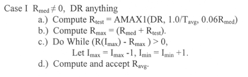
Note: This procedure has the effect of eliminating samples from the array used to compute the average until the largest value used in the average is within the median plus the expected 50% range given by Rtest. Here Rtest is taken to be the largest of the interquartile range, one count/average accumulation time, or 6 percent of the median. This is necessary to handle cases of very low count rate and nearly constant count rate. The 6% of median test is necessary because the 24 to 8 bit log compression of HISCALE rates produces discretization steps of this magnitude. Because the samples are eliminated in pairs, the median does not change during the procedure and does not need to be recomputed.

 

 

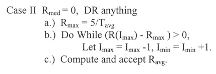
Note: For a set of samples with median value = 0, valid accumulations of counts exceeding 5 are very unlikely. The exact probability depends on fitting a binomial distribution precisely to the data. We do not believe that such fitting is necessary. Rather, we used representative cases of binomial distributions with trails and probabilities selected to produce success numbers similar to those experienced in the HISCALE data. The representative cases yielded occurrences of "5" very rarely, typically once per 10,000 trials.

 

4.) Validation of Quality Controlled Averaging

 

The QCA method has been applied to the HISCALE data shown in Figures A6-1 through A6-10. The QCA results are displayed in Figures A6-11 through A6-20. Visual inspection and comparison of the data "with" and "without" QCA shows the improvements achieved. Further information on the effect of QCA is provided at the end of this appendix; it shows a summary of the activity of the QCA procedure in excluding suspect data from the averages. The summary by rate channel (corresponding in order to the summary plots) shows the number of samples accepted and rejected (for Cases I, II). Note that the QCA procedure accommodates a wide variety of real trends in the data while excluding nearly every suspect point.

 

Figures:

 

• Figure A6-1 HISCALE hourly average of spin average rates, type 1, without QCA (E1' - FP6')
• Figure A6-2 HISCALE hourly average of spin average rates, type 2, without QCA (FP7' - P5')
• Figure A6-3 HISCALE hourly average of spin average rates, type 3, without QCA (P6' - W3)
• Figure A6-4 HISCALE hourly average of spin average rates, type 4, without QCA (W4 - Z2)
• Figure A6-5 HISCALE hourly average of spin average rates, type 5, without QCA (Z2A - E3)
• Figure A6-6 HISCALE hourly average of spin average rates, type 6, without QCA (E4 - P2)
• Figure A6-7 HISCALE hourly average of spin average rates, type 7, without QCA (P3 - P8)
• Figure A6-8 HISCALE hourly average of spin average rates, type 8, without QCA (DE1 - C WARTC)
• Figure A6-9 HISCALE hourly average of spin average rates, type 9, without QCA (D WARTD - F')
• Figure A6-10 HISCALE hourly average of spin average rates, type 10, without QCA (X-ray P1 - X-ray P2)
• Figure A6-11 HISCALE hourly average of spin average rates, type 1, with QCA (E1' - FP6')
• Figure A6-12 HISCALE hourly average of spin average rates, type 2, with QCA (FP7' - P5')
• Figure A6-13 HISCALE hourly average of spin average rates, type 3, with QCA (P6' - W3)
• Figure A6-14 HISCALE hourly average of spin average rates, type 4, with QCA (W4 - Z2)
• Figure A6-15 HISCALE hourly average of spin average rates, type 5, with QCA (Z2A - E3)
• Figure A6-16 HISCALE hourly average of spin average rates, type 6, with QCA (E4 - P2)
• Figure A6-17 HISCALE hourly average of spin average rates, type 7, with QCA (P3 - P8)
• Figure A6-18 HISCALE hourly average of spin average rates, type 8, with QCA (DE1 - C WARTC)
• Figure A6-19 HISCALE hourly average of spin average rates, type 9, with QCA (D WARTD - F')
• Figure A6-20 HISCALE hourly average of spin average rates, type 10, with QCA (X-ray P1 - X-ray P2)

 

5.) Plans for Production and Dissemination

 

Our plans are to add several steps to the production processing of HISCALE data with the currently processed QCA averages being included in routine shipments beginning in July 1993 (next month). A new data type is being defined that will be identical to the existing UAV file type but with a new external file name "UAFyyddd.LAN" and with internal identifiers in the record header history block. All HISCALE production software will be modified (slightly) to accept this new file name and to recognize UAF as opposed to UAV files in graphing. Note that only the ULAyyddd.RAT files get the QCA procedure applied.

 

As soon as possible, a QCA kit will be available for network copy to all HISCALE sites so that its use can begin immediately in analysis. Further, it is our intention to run UAF files for all HISCALE data from turn-on to the present. It is our goal to ship the results of this production in the form of 8 mm tapes of .UAF files for the entire period from turn-on up to the July 1993 shipment by the end of August 1993. The compute time for a 32 day period on our VAX STATION 4000/90 is about 2.5 hours on a dedicated machine. It will take a few weeks, therefore, to catch up.

 

---

Memo To: HISCALE Team
From: Tom Armstrong, Dennis Haggerty
Subject: Artifact in UAF data

 

The hourly and daily quality controlled averaged (QCA) rate files that we have shipped appear to have an error affecting the low count rates on a few channels. The good news is that this discovery explains the small periodic "square wave" that had appeared in some channels (P1' was the most conspicuous) and that we had feared might be due to instrumental effects aboard the spacecraft. From what we have done thus far to characterize and fix this problem, we see this effect only in the filtered averages. By comparing the unfiltered and filtered data plots, which often have different plot scales because of the presence of spurious high rates in the unfiltered data, we have initially attributed the lack of conspicuous effect in the unfiltered data to the much more compressed plotting scale. It turns out, however, that the periodic square wave is genuinely absent from the unfiltered data. The good news is that the instrument does not have a problem!!! The bad news is that the filtering process is doing something to the data that is very, very, subtle and that, while we are certain to be able to fix it, we will need to regenerate all of the hourly and daily filtered data from launch to the present. Fortunately, that only requires a week or so to accomplish--once we have tracked down this problem.

 

In case you are mystified by the above paragraph and haven't noticed the problem in your data plots, the effect is really small. It ranges from 0.1 c/sec downward to 0.005 c/sec. It is related to the spacecraft telemetry rate. Most likely it has to do with the way in which the filtered averages are weighted. It probably does not have to do with the criteria for excluding data because the effect is present even when the data quality is good and there is no noise. Dennis and I will find and fix this problem and report further on it.

 

Revisions as of August 4, 1993

 

1) The formulation of DR has been changed. Testing of the procedure has shown the greatest accuracy can be attained by using an interval DR = 10.0 * (R75% - R50%). The factor of 10.0 in the formulation is a weight parameter, determined by testing a large sample of data. This factor gave sufficient data filtering while allowing for very small events to be accurately averaged.

2) The rate blocks and the sectored timing blocks of the UAFyyddd.LAN files are in good agreement with those of the UAVyyddd.LAN files. The duty cycles of the UAFyyddd.LAN will be equal to or slightly smaller than the duty cycles contained in the UAVyyddd.LAN files. The product of the sectored timing block and the duty cycle will reflect the correct instrument 'on time', after filtering has occurred.

 

Activity Log of Data Filter, 93-JUN-28

 

 

Return to HISCALE List of Appendices

Return to Ulysses HISCALE Data Analysis Handbook Table of Contents

 

QUICK FACTS

RELATED LINKS