4.9 Modeling of the Magnetic Electron Deflection System

 

4.9.1 Without Scattering

 

The following section summarizes the results of John Buckley's thesis, “Geometric Factor Study for the Deflected Electrons of HISCALE, the Heliosphere Instrument for Spectrum, Composition and Anisotropy at Low Energies.” The complete thesis is included as an appendix.

For the deflected electrons of HISCALE, the detector is able to distinguish between four separate energy ranges labeled DE1 through DE4. Table 4.18 lists the current values used for these passbands. It also shows the resulting geometric factors obtained for the passbands for the Trial 10 B-field.

 

Table 4.18 Geometric factors for deflected electrons trial 10 B-field

 

Energy Channel	Ehi (keV)	Elo (keV)
DE1	53	38
DE2	103	53
DE3	175	103
DE4	315	175

 

During the course of this study, a total of three different geometries and four magnetic fields were used. The first geometry adopted was missing a notch that was later filed in the actual flight instrument. Results for this are not discussed here. The second and the third geometries are both similar versions of the geometry with the notch included. For each of the latter two geometries, four slightly different magnetic fields were used to determine the geometrical factors. The resulting plots of G vs. E are shown in Figure 4.75, and Table 4.19 gives the geometric factors for the four energy channels averaged over all eight trials.

 

Figure 4.75 Plots of G vs. E for all eight trials

 

 

 

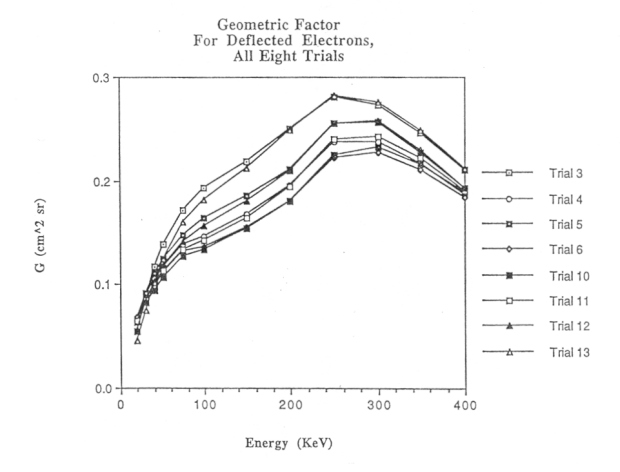
Table 4.19 Deflected electron geometrical factors

 

The current values used in the production program of the HISCALE instrument are summarized in a data file IDF.DAT. Also listed in Table 4.19 are the IDF.DAT values of the geometric factors for the deflected electrons. As one observes from the table, there are certainly some discrepancies between the two sets of values. These and other problems are discussed below.

 

Testing results with experimental data. The fact that HISCALE has other detectors that also count electrons provides a means of checking the calculated G-factors. One way of doing this is to simply compare the fluxes of the deflected electrons with the other electron energy channels. In particular, HISCALE also has the two foil detectors mentioned previously that detect electrons at low energies for specified passbands. These channels and their passbands are presented in Table 4.20.

 

Table 4.20 LEFS60 and 150 electron passbands

 

 

In order to compare one channel with the another, it is necessary to first adjust the passband of one of the two channels to fit the passband of the other. This can only be done if channels adjacent to the ones of interest exist, which they do in this case. The approximation is also most valid for passbands that overlap fairly well to begin with. Once this passband adjustment of the raw count rates is made, and the results are divided by the corresponding GDE, then the resulting ratios are electron fluxes from the different detectors. If one is dealing with an isotropic event, the resulting electron fluxes should all be the same. Figure 4.76a shows such a comparison for the IDF.DAT version of the G-factors for an electron event occurring on day 301 of 1991. The agreement between the channels is good, as indicated by the close overlap of each line with the other. Figure 4.76b shows the same plot, except now the calculated values of G from Trial 10 are used. The agreement is not as good, as can be seen from the poor overlap of the spectra. In fact, it appears that for passband DE1, the geometric factor has been underestimated, and for DE4 it has been overestimated. Figure 4.76c shows the spectra for the same event using the average G-factors of all eight trials. The overlap is worse than before. In doing such a comparison, one must be careful to:

 

1. Be sure the electron event is an isotropic one--the telescopes of HISCALE all point in different directions at any given time.

 

2. Be careful of the possibility of heavy ion and proton contamination of the lower energy LEFS-channels, i.e., one should look at the purely electron events.

 

3. Be aware that there may be an energy-dependent foil factor for the LEFS, and that without its inclusion the comparison could be invalid.

 

• Figure 4.76a Spectra plots for the DE and two LEFS channels using IDF.DAT G-factors
• Figure 4.76b Spectra plots for the same time period using Trial 10 G-factors
• Figure 4.76c Spectra plots for the same time period using Table 4.18 G-factors

 

Another means of comparing these channels is to take the ratio of the passband adjusted count rates without converting them to fluxes. Then if the event occurs during an isotropic time period, the ratio should simply be the quotient of geometric factors of LEFS vs. DE channels. For example, let’s say we take the ratio of E1 to DE1 fluxes, where a passband adjustment has been made to RDE1 (which means that DE1 = DE2). If the time is indeed an isotropic one, then the fluxes should be the same, and the ratio is of value 1:

 

Flux (E1) / Flux (DE1) = (RE1/GE1DE) / (RDE1 (adj)/GDE1DE = 1

 

A little algebra shows that

 

RE1/RDE1 (adj) = GE1/GDE1

 

Thus, if we know the geometric factor for the LEFS channels, we can determine G for the DE's. In fact, because of the simple cylindrical symmetric geometry of the LEFS telescope, the G-factors of the LEFS channels are known and believed to be highly accurate. Figure 4.77a shows the above ratio for the four different energy channels over a 32 day period in 1991. The dotted line represents the anticipated ratio using the IDF.DAT values, whereas the dashed line gives the anticipated simulation ratio (see Table 4.19). As one can deduce from the plots, the IDF.DAT values give much better agreement for channels DE1 and DE4 during this time period. However, for the DE2 and DE3 channels, it appears that both the simulation and IDF.DAT values for G are overestimated, and need to be smaller. For example, using the data of days 93 and 94 of 1991, we can deduce from the ratio plots that G for DE2 is about .12 cm2sr, and for DE3 the G-factor should be .08 cm2sr.

 

Of course, one must be careful when doing such an estimate; ion contamination is often present in the LEFS channels. Figure 4.77b shows ratio plots for a later time period in 1991; note how the ion event on and around day 186 affects the higher energy channels. Ion contamination in these channels gives an inflated ratio. Also, low counting rates near the noise level can give ambiguous results. Because of these possibilities, one desires to look at these ratio plots during a high density electron event. Figure 4.77c reveals the electron event around day 301 discussed earlier. Once again, the IDF.DAT values for G appear to be better estimates for the DE1 and DE4 energy channels, the other two being overestimated as before.

 

• Figure 4.77a Ratio plots for all four energy channels for a 32-day period.
• Figure 4.77b Ratio plots for a later time period in 1991.
• Figure 4.77c Ratio plots including the electron event around day 301.
• Figure 4.77d Ratio plots for a 32-day period in 1992.  

 

Up to now it appears that the ratio plots support the IDF.DAT values for G over simulation values. But as Figure 4.77d shows for a time period in 1992, sometimes these ratio plots can be deceiving.

 

It appears that the calculated G-factors are in general good approximations, but lack consistency with experimental data. Primary reasons for the discrepancies are believed to come from scattering effects, and overall efficiency factors that the model cannot account for.

 

Absolutely no scattering is taken into account in this simulation, primarily because the very nature of the scattering is complex and in most cases impossible to include due to lack of information. Unwanted scattering of electrons can cause electrons to hit and register on the detector that would not normally make it there.

 

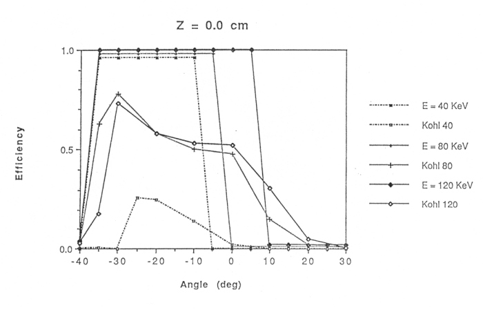
The other flaw in the model is the fact that it assumes 100% counting efficiency for the detector. That is, if an electron makes it through the telescope to the detector surface, the simulation automatically assumes that the detector counts the hit. But in reality, not all electrons making it to the detector end up registering as a count. To put it another way, the simulation assumes 100% counting efficiency, whereas in reality this is rarely the case. Before the flight instrument was launched, a calibration was done to determine the electron counting efficiency for an electron beam coming in at various angles and positions from Shodhan's* y-axis. Figure 4.78 compares calibration results with the simulation. As one can see, the overall angle ranges where electrons make it to the detector are fairly consistent, but the absolute efficiencies are always overestimated in the simulation. It turns out that the efficiency of any slab-like detector is going to depend not only on electron energy, but also the angle at which the electron intercepts the detector.

 

(*S. Shodhan master's thesis, Univ. of Kansas, 1988)

 

Figure 4.78 A plot comparing Kohl's electron efficiency study with the simulation. Note how angular cutoff positions match up, but overall values for nonzero efficiencies cannot be accounted for with the simulation.

 

 

In conclusion, the results of this study of the geometric factor of the deflected electrons for the Ulysses HISCALE instrument reveal that the simulation is not sufficiently accurate to give reliable values. More reliable are the ratio and the spectra plots that use actual data and involve all three counting instruments aboard HISCALE.

 

 

4.9.2 With Scattering (Xiaodong Hong Thesis)

 

Please refer to Appendix 10.

 

 

Next: Chapter 4.10 Many-fold Coincidence Pileup in Silicon Detectors:  Solar X-Ray Response of Charged Particle Detector Systems for Space (manuscript by Nikitin et al.)